Training and hyperparameter optimization¶

Introductory notes¶

ADMET-XSpec is a tool that seeks to allow researchers to investigate the viability of integrating non-human assays into the human drug development process, specifically with respect to ADMET properties. It is worthwhile to keep this in mind when considering major elements of how the tool functions, including:

Aggregating splits during training
Filtering using Tanimoto distance to the test set
Using an “arbitrary” binary classification threshold of the mean or median of human regression values

In short, we want to try out as many methods of enriching the training set - normally composed of solely human data - with mouse and rat data. If performance worsens, we want to amend our approach (filtering). If establishing a “proper” source of truth for classification is not necessary (a unanimously agreed-upon value for inactivity vs. activity), we simply want to see if classification accuracy improves when adding new data (using the mean or median of regression values as the classification threshold).

Sections¶

How the raw data is transformed before it ends up in the training loop (preprocessing)
ScikitPredictorBase as the model-training interface & optimizing training
Where to find outputted models

How the raw data is transformed¶

Goals¶

After reading this section, you will understand all of the transformations applied to the data before it ends up in a training loop for an ML method.

Let’s base our discussion on a diagram that illustrates the flow of data:

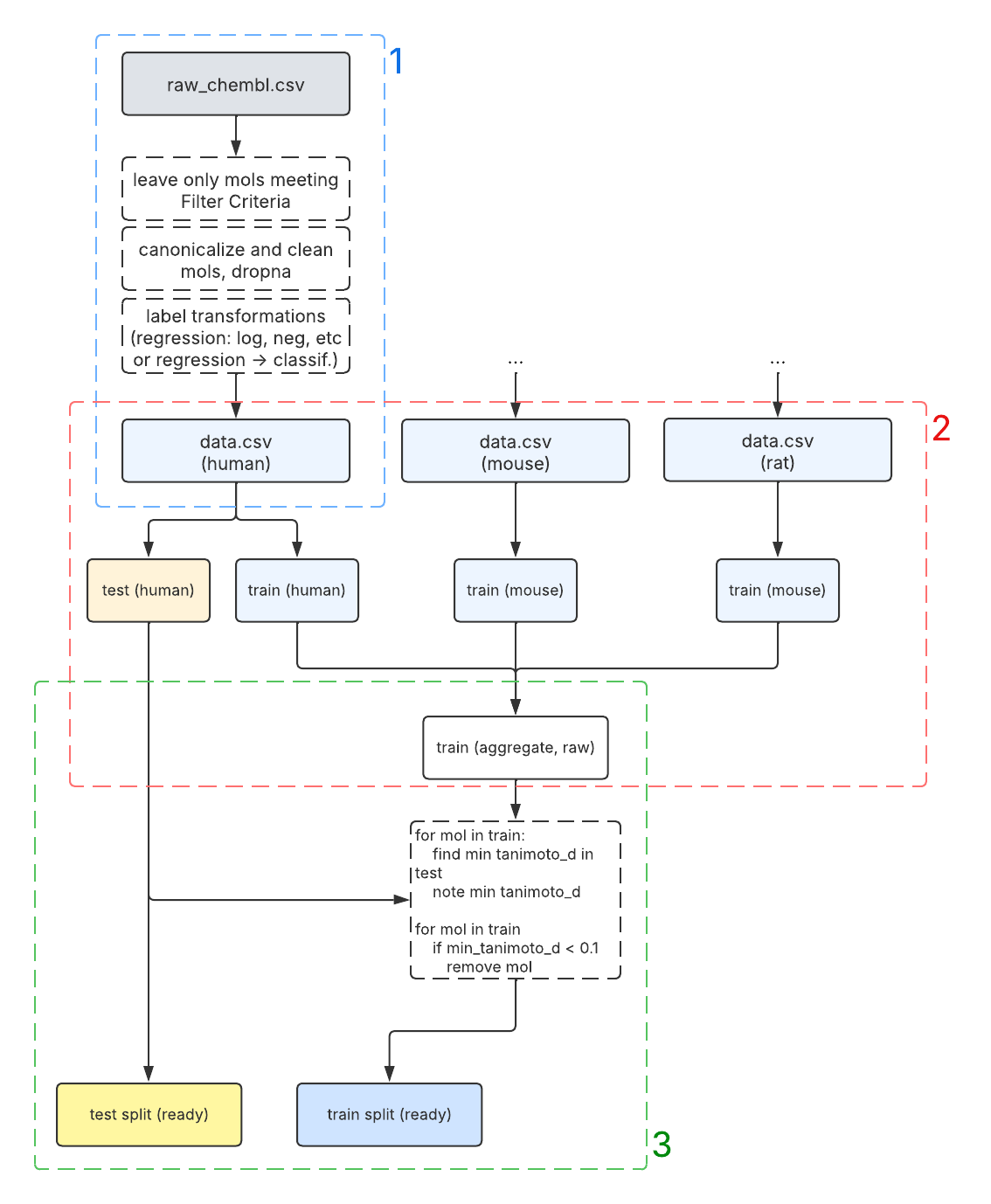
This diagram shows how we take raw ChEMBL human, mouse, and rat data and provide it to model training classes implementing the ScikitPredictorBase interface.

Let’s briefly note the 3 color-coded sections, which group together concerns at the different stages of data transformation:

Arriving at the prepared dataset. This is mostly accomplished by the DataInterface class.
Splitting the prepared human data and integrating rodent data to form the test set (final) and aggregate train set (raw). This is accomplished with ProcessingPipeline relying on DataInterface for data loading operations and weaving in some of its own manipulations.
Filtering the aggregate train set by minimum Tanimoto distance to molecules in the test set. This is best explained by the pseudocode for loop in the diagram and is achieved through using SimilarityFilterBase in ProcessingPipeline.

Arriving at the prepared dataset¶

Recall these parts of AChE/human/regression/params.yaml:

 filter_criteria:
     Standard Units:
       - "nM"
     Standard Relation:
      - "'='"
    Standard Type:
      - "IC50"
label_transformations:
  - "log10"
  - "negate"

and these parts in AChE/human/binary_classification/params.yaml:

5.  task_setting: "binary_classification"
6.  threshold: "median"

You can think of these parameters as “hard-coded” filters that you apply to a raw dataset included in data/datasets. By the time the data reaches the boundary of 1: Arriving at the prepared dataset and enters 2: Splitting the prepared human data, it is guaranteed to have the following qualities:

Only those molecules in the ChEMBL .csv that met the standard unit, standard value, and (if applicable) standard
relation criteria remain; in the case of transforming to binary classification, only those that could be
unambiguously placed in either the inactive or active category (appropriate < or > values)
Of those molecules, only those whose SMILES passed canonicalization remain; for the exact details of this step,
see get_clean_smiles in src.utils
For those molecules, the label transformations have been applied in the regression setting, and in the binary
classification setting, the labels have been converted to 0 (inactive) or 1 (active)

Before proceeding to the next section, the SMILES are featurized. For the sake of example, we assume that the ECFP4 fingerprint featurizer is employed.

Splitting the prepared human data, integrating rodent data¶

(description of scaffold splitting and its motivation…)

Filtering the aggregate train set by minimum Tanimoto distance¶

(description of filtering by Tanimoto and its motivation…)

`ScikitPredictorBase` as the model-training interface & optimizing training¶

Goals¶

After reading this section, you will understand how we use scikit-learn’s well-established interface to train models, as well as how we run optimization and save optimized hyperparameters, which can be used for future runs.

You will also know where to find the configs responsible for the ranges and distributions from which we sample hyperparameters for the optimization search.

ScikitPredictorBase exposes the following public methods:

def train(self, smiles_list, target_list)
def optimize(self, smiles_list, target_list)
def predict(self, smiles_list):
def get_hyperparameters(self):
def set_hyperparameters(self, params)

Where to find outputted models¶

Goals¶

After reading this section, you will understand the contents of a successful training run outputted to data/cache.

Models are outputted to data/cache/models. Let’s look at an example of the result of a ProcessingPipeline run that successfully trained a model:

LightGBM_clf_ecfp_featurizer_4b52a
└── scaffold_e4737_tanimoto_5p_filter_c2805_91da5
	├── hyperparams.yaml
	├── metrics.yaml
	├── model_final_refit.pkl
	├── model_metadata.yaml
	├── model.pkl
	├── operative_config.gin
	└── training_log
		└── console.log

You can think of them as follows:

train trains a model based on a set of data and internal hyperparameters. These are provided through an experiment_config.gin (the filename is used as an example).

optimize performs a RandomizedSearchCV (scikit docs) to train a model (and discard it) and save the optimal hyperparameters internally. If train were run now, the model would be trained with those optimal hyperparameters.

predict returns a list of predictions: probability of the positive class for classifiers and predicted values for regressors. This can be used to collect metrics about the fit.

get_hyperparameters retrieves the hyperparameters stored within the class. set_hyperparameters sets those hyperparameters.

Here are 3 use cases of the ProcessingPipeline that motivate these methods:

Simply training a model with predefined experiment_config.gin parameters and outputting it to ./data/cache/models
Finding optimal hyperparameters by having optimize find them, and then training a model on those parameters (in this case, we provide ranges and distributions for sampling the hyperparameters; more on this further down this section)
Training a model on optimal hyperparameters without finding them with optimize—instead, loading optimal hyperparameters that were saved to disk

These various use cases are covered by different processing_plans, which we covered earlier.

The configs governing the hyperparameter search space can be found under: ./configs/predictors/classifiers/optimization/*_hyperparams.gin and ./configs/predictors/regressors/optimization/*_hyperparams.gin.

Here is the part covering the distribution for LGBM as an example:

LightGbmClassifier.params_distribution = {
    'n_estimators': @n_estimators/QLogUniform(),
    'max_depth': @max_depth/QUniform(),
    'num_leaves': @num_leaves/QUniform(),
    'min_child_samples': @min_child_samples/QUniform(),
    'learning_rate': [0.01, 0.05, 0.1],
}

Where to find outputted models¶

Goals¶

After reading this section, you will understand the contents of a successful training run outputted to data/cache.

Models are outputted to data/cache/models. Let’s look at an example of the result of a ProcessingPipeline run that successfully trained a model:

LightGBM_clf_ecfp_featurizer_4b52a
└── scaffold_e4737_tanimoto_5p_filter_c2805_91da5
	├── hyperparams.yaml
	├── metrics.yaml
	├── model_final_refit.pkl
	├── model_metadata.yaml
	├── model.pkl
	├── operative_config.gin
	└── training_log
		└── console.log

The directory name for the model is composed of:

The model name: LightGBM_clf (a classifier in this case)
The featurizer name: ecfp_featurizer
The featurizer’s “hash code,” a result of MD5 hashing its parameters: 4b52a

The directory name for the data that resulted in this model being trained (one model can have multiple such subdirectories) follows suit and is composed of:

The splitter key, which contains the splitter type and hash code: scaffold_e4737
The filter key, again with the hash code: tanimoto_5p_filter_c2805
The datasets hash code: 91da5

All of this hashing is done to aid tracking of models in a more organized way than simply appending the date to their name. As you can see in the example, there is plenty of metadata to go along with this technique, which has already been covered in section 1.2.

Training and hyperparameter optimization¶

Introductory notes¶

Sections¶

How the raw data is transformed¶

Goals¶

Arriving at the prepared dataset¶

Splitting the prepared human data, integrating rodent data¶

Filtering the aggregate train set by minimum Tanimoto distance¶

ScikitPredictorBase as the model-training interface & optimizing training¶

Goals¶

Where to find outputted models¶

Goals¶

Where to find outputted models¶

Goals¶

`ScikitPredictorBase` as the model-training interface & optimizing training¶